Sums of Powers of Integers, using Forced Induction (Generative Induction)

SiteMap of SciRealm | About John | John's Resume/C.V./Bio | Send email to John John's Science, Math, Philosophy Stuff: The Science Realm: John's Virtual Sci-Tech Universe | 4-Vectors | Ambigrams | Antipodes | Covert Ops Fragments | Cyrillic Projector | Forced Induction (Sums Of Powers Of Integers) | Fractal Tree | Frontiers | IFS Fractals (Assembly) | IFS Fractals (Javascript) | JavaScript Graphics | Kid Science | Kryptos | Philosophy | Photography | Physics-Planck Constant Measurement Via LEDs | Prime Sieve | QM from SR | QM from SR-Simple RoadMap | QM from SR-Simple RoadMap (PDF) | SR 4-Vector & Tensor Calculator |Quantum Phase | Quotes | RuneQuest Cipher Challenge | Secret Codes & Ciphers | Scientific Calculator (complex capable) | Science+Math | Sci-Pan Pantheist Poems | Stereograms | SuperMagicSqr4x4 |Turkish Grammar |Melike Wilson Art Site last modified: 2021-Aug	Welcome to Relativistic Quantum Reality: Virtual worlds of imaginary particles: The dreams stuff is made of: Life, the eternal ghost in the machine... This site is dedicated to the quest for knowledge and wisdom, through science, mathematics, philosophy, invention, and technology.  May the treasures buried herein spark the fires of imagination like the twinkling jewels of celestial light crowning the midnight sky... 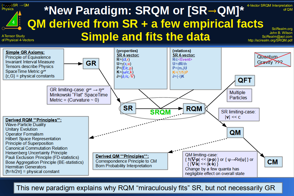Quantum Mechanics is derivable from Special Relativity See SRQM - QM from SR - Simple RoadMap (.html) See SRQM - QM from SR - Simple RoadMap (.pdf) See SRQM - Online SR 4-Vector & Tensor Calculator See Online Complex-capable RPN Scientific Calculator ***Learn, Discover, Explore***

METHOD OF FORCED INDUCTION (or GENERATIVE INDUCTION)
used to calculate the Sums of Powers of Integers

N
Sum[ x ⁿ ]
x=1

Normally, the method of induction is used to logically prove that a given mathematical or symbolic relation is true, after the relation has already been found by other methods. However, in this analysis, the method of Forced Induction (or Generative Induction) will be introduced to force a relation to be true. When used to calculate the sum of integers to a given power, the result it gives is very powerful and quite elegant. It basically generates the general expression for the sum of integers to any positive integer power. I have never seen the general expression from any other method.


Notes/Usage:
N = # of terms in the sum
n = power of the integers in the sum
Sum[xⁿ] = Summation function over the given indices
Binom[a,b] = Binomial function = a!/[b!(a-b)!)]
LHS = Left-Hand Side, RHS = Right-Hand Side
delta function d^ab = { 0 if a<>b; 1 if a=b }

N
Sum[ x ] = N²/2+N/2
x=1

Mathematical Induction can be used in the following manner to prove this relation true.

Step 1: Show that the first case is true. So, set N equal to 1.

 1
Sum[ x ] = 1²/2+1/2
 x=1

1 = 1/2+1/2

1 = 1 True!

Step 2: Show that the subsequent cases are true. So, set N to the value N+1.

 N+1
Sum[ x ] = (N+1)²/2+(N+1)/2
 x=1

 N
Sum[ x ]+(N+1) = [(N²+2N+1)+(N+1)]/2
 x=1

(N²/2+N/2)+(N+1) = (N²/2+3N/2+1)

(N²/2+3N/2+1) = (N²/2+3N/2+1)

Proof Complete!

Therefore, the relation is also true for all integer values greater than 1; N=1 proves N=2, N=2 proves N=3, N=3 proves N=4, etc. assuming that N=1 is true, which was shown in the first step. Thus, in the last step, the formula is proven true for all positive integers. This is the manner in which standard method of induction is used.

N
Sum[ x ] = N²/2+N/2
x=1

 1000
Sum[ x ] = 1000²/2+1000/2 = 500500
 x=1

N                 3
Sum[ x² ] = Sum[ c_i Nⁱ ] = c₁ N¹+c₂ N²+c₃ N³
x=1              i=1

where the c_i's are constants to be determined.

Step 1: Force the first case to be true. So, set N equal to 1.

 1
Sum[ x² ] = c₁ 1¹+c₂ 1²+c₃ 1³
 x=1

1² = c₁ 1¹+c₂ 1²+c₃ 1³

1 = c₁+c₂+c₃

so the sum of the c_i's equals 1.

Step 2: Force the subsequent cases to be true. So, set N to the value N+1.

 N+1
Sum[ x² ] = c₁ (N+1)¹+c₂ (N+1)²+c₃ (N+1)³
 x=1

 N
Sum[ x² ]+(N+1)² = c₁ (N+1)¹+c₂ (N+1)²+c₃ (N+1)³
 x=1

c₁ N¹+c₂ N²+c₃ N³+(N+1)² = c₁ (N+1)¹+c₂ (N+1)²+c₃ (N+1)³

c₁ (N+1)¹+c₂ (N+1)²+c₃ (N+1)³-c₁ N¹-c₂ N²-c₃ N³ = (N+1)²

c₁ N¹+c₁+c₂ N²+2c₂ N+c₂+c₃ N³+3c₃ N²+3c₃ N+c₃-c₁ N¹-c₂ N²-c₃ N³ = N²+2N+1

c₁+2c₂ N+c₂+3c₃ N²+3c₃ N+c₃ = N²+2N+1

Now let's rewrite the last equation in terms of the powers of N.

(3c₃-1) N²+(2c₂+3c₃-2) N¹+(c₁+c₂+c₃-1) N⁰ = 0

Now then, we want the last equation to hold for any value of N. Therefore, one must set the coefficients of the N's to zero separately. For this case, that will give us 3 equations to solve. Let's rewrite the equations to a nicer [matrix] form.

                3c₃ = 1
        2c₂+3c₃ = 2
1c₁+1c₂+1c₃ = 1

One now has an already matrix-triangulized set of linear equations for the c_i's which are independent of the value of N. Also note that condition from step 1 is satisfied automatically by the last equation. These equations are easily solved to give: c₁=1/6, c₂=1/2, c₃=1/3
Therefore, the sum of squared integers is:

N
Sum[ x² ] = N³/3+ N²/2+ N¹/6
x=1

This equation is True for all integers N>=1 by construction using the method of forced induction.

N                  n+1 Sum[ x n ] = Sum[ ci Ni ]  x=1               i=1

Step 1: Force the first case to be true. So, set N equal to 1.

 1                  n+1
Sum[ x ⁿ ] = Sum[ c_i 1ⁱ ]
 x=1               i=1

         n+1
1ⁿ = Sum[ c_i ]
         i=1

 n+1
Sum[ c_i ] = (c₁+c₂+ ... + c_n+1) = 1
 i=1

As before, the sum of the c_i's must equal 1.

Step 2: Force the subsequent cases to be true. So, set N to the value N+1.

 N+1              n+1
Sum[ x ⁿ ] = Sum[ c_i (N+1)ⁱ ]
 x=1               i=1

 N                               n+1
Sum[ x ⁿ ]+(N+1)ⁿ = Sum[ c_i (N+1)ⁱ ]
 x=1                            i=1

n+1                      N
Sum[ c_i (N+1)ⁱ ]-Sum[ x ⁿ ] = (N+1)ⁿ
i=1                       x=1

Using the assumed solution form on the middle term:

n+1                      n+1
Sum[ c_i (N+1)ⁱ ]-Sum[ c_i Nⁱ ] = (N+1)ⁿ
i=1                       i=1

n+1
Sum[ c_i ( (N+1)ⁱ - Nⁱ ) ] = (N+1)ⁿ
i=1

Using the binomial expansion on the LHS:

n+1          i
Sum[ c_i (Sum[ Binom[i,j] N^j ] - Nⁱ) ] = (N+1)ⁿ
i=1          j=0

n+1         i-1
Sum[ c_i (Sum[ Binom[i,j] N^j ] + Binom[i,i] Nⁱ - Nⁱ) ] = (N+1)ⁿ
i=1          j=0

n+1         i-1
Sum[ c_i (Sum[ Binom[i,j] N^j) ] = (N+1)ⁿ
i=1          j=0

Using the binomial expansion on the RHS:

n+1         i-1                                  n
Sum[ c_i (Sum[ Binom[i,j] N^j) ] = Sum[ Binom[n,k] N^k]
i=1         j=0                                  k=0

Now expand in terms of powers of N:

n+1
Sum[ c_i (Binom[i,0] N⁰ + Binom[i,1] N¹ +...+ Binom[i,i-1] N^i-1) ] = Binom[n,0] N⁰ + Binom[n,1] N¹ + ... + Binom[n,n] Nⁿ
i=1

Again, one gathers the terms for each power of N (I have left out the exact indices...):

(Binom[n,0]-Sum[ c_i (Binom[i,0] )) N⁰ + (Binom[n,1]-Sum[ c_i (Binom[i,1])) N¹ + ... + (Binom[n,n]-Sum[ c_i (Binom[i,i-1])) N^i-1 = 0

Again, the coefficients of each power of N must equate to zero separately, and then one obtains the following (n+1) relations labeled by j=[0..n]:

n+1 Sum[ Binom[i,j] * ci ] = Binom[n,j]  for j=[0..n] i=j+1

These relations are an already matrix-triangulized set of linear equations for the c_i's. They are easy to solve, especially if one starts with the (j=n) equation and works down to the (j=0) equation. Again, the (j=0) equation says that the sum of the c_i's must equal 1, in agreement with the first condition. Now, let us say that one wants to sum the first N integers to the 3^rd power. We will use the relations given by the forced induction. Note that n=3 for the sum of cubes.

 3+1
Sum[ Binom[i,j] c_i ] = Binom[3,j]  for j=[0..3]
 i=j+1

For (j=3) we get:

Binom[4,3] c₄ = Binom[3,3]

4c₄ = 1

c₄ = 1/4

For (j=2) we get:

Binom[3,2] c₃ + Binom[4,2] c₄ = Binom[3,2]

3c₃ + 6(1/4)= 3

c₃ = 1/2

For (j=1) we get:

Binom[2,1] c₂ + Binom[3,1] c₃ + Binom[4,1] c₄ = Binom[3,1]

2c₂ + 3(1/2) + 4(1/4)= 3

c₂ = 1/4

For (j=0) we get:

Binom[1,0] c₁ + Binom[2,0] c₂ + Binom[3,0] c₃ + Binom[4,0] c₄= Binom[3,0]

c₁ + (1/4) + (1/2) + (1/4) = 1

c₁ = 0

Thus, the sum of cubed integers is:

N
Sum[ x³ ] = N⁴/4+ N³/2+ N²/4
x=1

 Binom[n+1,n] c_n+1 = Binom[n,n]

[(n+1)n!] c_n+1 / [n!1!] = 1

c_n+1 = 1/(n+1)

For (j=n-1) we get (using the result from above):

 Binom[n,n-1] c_n + Binom[n+1,n-1] c_n+1 = Binom[n,n-1]

[n(n-1)!] c_n / [(n-1)!1!] + [(n+1)n(n-1)!] [1/(n+1)] / [(n-1)!2!] = [n(n-1)!] / [(n-1)!1!]

n c_n + n/2 = n

c_n = 1/2

For (j=n-2) we get (using the results from above):

 Binom[n-1,n-2] c_n-1 +Binom[n,n-2] c_n + Binom[n+1,n-2] c_n+1 = Binom[n,n-2]

[(n-1)!] c_n-1 / [(n-2)!1!] +[n!] c_n / [(n-2)!2!] + [(n+1)!] c_n+1 / [(n-2)!3!] = [n!] / [(n-2)!2!]

[(n-1)(n-2)!] c_n-1 / [(n-2)!1!] +[n(n-1)(n-2)!] c_n / [(n-2)!2!] + [(n+1)n(n-1)(n-2)!] c_n+1 / [(n-2)!3!] = [n(n-1)(n-2)!] / [(n-2)!2!]

[(n-1)] c_n-1 / [1!] +[n(n-1)] c_n / [2!] + [(n+1)n(n-1)] c_n+1 / [3!] = [n(n-1)] / [2!]

[(n-1)] c_n-1 / [1] +[n(n-1)] [1/2] / [2] + [(n+1)n(n-1)]  / [(n+1)][6] = [n(n-1)] / [2]

[(n-1)] c_n-1 / [1] +[n(n-1)] / [4] + [(n+1)n(n-1)]  / [(n+1)][6] = [n(n-1)] / [2]

c_n-1 / [1] +[n] / [4] + [(n+1)n]  / [(n+1)][6] = [n] / [2]

c_n-1 +[n/4] + [(n+1)n]  / [6(n+1)] = [n/2]

c_n-1 +[n/4] + [n/6] = [n/2]

c_n-1 = n/12

and so forth. The following are the generalized coefficients c_i, found by solving the matrix-triangulized linear equations from above, starting with the (j=n) equation and working down towards the (j=0) equation:

c_n+1 = 1/(n+1)
c_n = 1/2
c_n-1 = n/12
c_n-2 = 0
c_n-3 = -n(n-1)(n-2)/720
c_n-4 = 0
c_n-5 = n(n-1)(n-2)(n-3)(n-4)/30240
c_n-6 = 0
c_n-7 = -n(n-1)(n-2)(n-3)(n-4)(n-5)(n-6)/1209600
c_n-8 = 0
c_n-9 = n(n-1)(n-2)(n-3)(n-4)(n-5)(n-6)(n-7)(n-8)/47900160
c_n-10 = 0
c_n-11 = -n(n-1)(n-2)(n-3)(n-4)(n-5)(n-6)(n-7)(n-8)(n-9)(n-10)/13076743680000
c_n-12 = 0
etc.

Thus, one finds that the general formula for sums of powers of integers is:

N Sum[ xn ] = (1/(n+1)) Nn+1 + (1/2) Nn + (n/12) Nn-1 + (0) Nn-2 + (-n(n-1)(n-2)/720) Nn-3 + (0) Nn-4 +...+ (.?.) N1 x=1

where the final term in a given series is the first power of N term (.?.) N¹.

Thus, there are (n+1) terms in a given series, although some of the coefficients may be zero (about half of them in fact).

So what would be the sum of integers to the 4^th power? In that case, n=4. There will be (4+1=5) coefficients.

c₄₊₁ = c₅ = 1/(4+1) = 1/5
c₄    = c₄ = 1/2
c_4-1 = c₃ = 4/12 = 1/3
c_4-2 = c₂ = 0
c_4-3 = c₁ = -4(4-1)(4-2)/720 = (-4)(3)(2)/720 = -24/720 = -1/30

N
Sum[ x⁴ ] = N⁵/5+N⁴/2+N³/3-N/30
x=1

Looking at patterns in the previous formulas gives the following relations (no proof given, but it seems to work):

cj+1[n] = c1[n-j] * Binom[n,j] / (j+1)  for j=[0..n]

Combining this relation with the last term coefficients, {c₁[n]}, gives another way to build the formulas:

c₁[n=0] = 1/(0+1) = 1
c₁[n=1] = 1/2
c₁[n=2] = 2/12 = 1/6
c₁[n=3] = 0
c₁[n=4] = -4(4-1)(4-2)/720 = (-4)(3)(2)/720 = -1/30
c₁[n=5] = 0
c₁[n=6] = 6(6-1)(6-2)(6-3)(6-4)/30240 = (6)(5)(4)(3)(2)/30240 = 1/42
c₁[n=7] = 0
c₁[n=8] = -8(8-1)(8-2)(8-3)(8-4)(8-5)(8-6)/1209600 = (-8)(7)(6)(5)(4)(3)(2)/1209600 = -1/30
c₁[n=9] = 0
etc., but here are a few more just for fun...
c₁[n=10] = 5/66
c₁[n=11] = 0
c₁[n=12] = -691/2730
c₁[n=13] = 0
etc.

c_j+1[5] =...........=  c₁[5-j] * Binom[5,j] / (j+1)  for j=[0..5]

c₅₊₁[5] = c₆[5] = c₁[5-5] * Binom[5,5] / (5+1) = c₁[0] * Binom[5,5] / (6) = (1) * 1 / 6 = 1/6
c₄₊₁[5] = c₅[5] = c₁[5-4] * Binom[5,4] / (4+1) = c₁[1] * Binom[5,4] / (5) = (1/2) * 5 / 5 = 1/2
c₃₊₁[5] = c₄[5] = c₁[5-3] * Binom[5,3] / (3+1) = c₁[2] * Binom[5,3] / (4) = (1/6) * 10 / 4 = 5/12
c₂₊₁[5] = c₃[5] = c₁[5-2] * Binom[5,2] / (2+1) = c₁[3] * Binom[5,2] / (3) = (0) * 10 / 3 = 0
c₁₊₁[5] = c₂[5] = c₁[5-1] * Binom[5,1] / (1+1) = c₁[4] * Binom[5,1] / (2) = (-1/30) * 5 / 2 = -1/12
c₀₊₁[5] = c₁[5] = c₁[5-0] * Binom[5,0] / (0+1) = c₁[5] * Binom[5,0] / (1) = (0) * 1 / 1 = 0

N
Sum[ x⁵ ] = N⁶/6+N⁵/2+5N⁴/12-N²/12
x=1

Relations based on differences between successive formulas gives

c₁[0]=1
              n+1
c₁[n]=1-Sum[ c_j[n] ] ; c_j[n]=(n / j) c_j-1[n-1] for j=[2..n+1]
              j=2

Another way to say this: To get the n^th sum:
Integrate the (n-1)^th sum formula;
Multiply all terms by n;
Add a term c₁[n]*N such that the sum of the c_i[n]'s = 1

...

Combining all these relations gives the recursion relation for the c₁'s:

              n
c₁[n]=1-Sum[ c₁[n-j]*Binom[n,j] / (j+1) ]
              j=1

Rewriting gives:

c1[0] = 1

n-1 c1[n] = 1 - Sum[ c1[k] * Binom[n+1,k] ] / (n+1)                   k=0

B0 = 1

n-1 Bn = - Sum[ Binom[n+1,k] * Bk ] / (n+1)             k=0

c₁[n=0] = B₀ = 1
c₁[n=1] = 1/2    **(B₁ = -1/2)**
c₁[n=2] = B₂ = 1/6
c₁[n=3] = B₃ = 0
c₁[n=4] = B₄ = -1/30
c₁[n=5] = B₅ = 0
c₁[n=6] = B₆ = 1/42
c₁[n=7] = B₇ = 0
c₁[n=8] = B₈ = -1/30
c₁[n=9] = B₉ = 0
c₁[n=10] = B₁₀ = 5/66
c₁[n=11] = B₁₁ = 0
c₁[n=12] = B₁₂ = -691/2730
c₁[n=13] = B₁₃ = 0
etc.

c1[0] = 1

n-1 c1[n] = 1 - Sum[ Binom[n+1,k] * c1[k] ] / (n+1)                   k=0

The Sum Integer Power recursion is just 1+Bernoulli recursion
This is the reason for c₁[n=1]=(+1/2) and B₁=(-1/2)

N
Sum[ x⁰ ] = N
x=1

N
Sum[ x¹ ] = N²/2+N/2
x=1

N
Sum[ x² ] = N³/3+N²/2+N/6
x=1

N
Sum[ x³ ] = N⁴/4+N³/2+N²/4
x=1

N
Sum[ x⁴ ] = N⁵/5+N⁴/2+N³/3-N/30
x=1

N
Sum[ x⁵ ] = N⁶/6+N⁵/2+5N⁴/12-N²/12
x=1

N
Sum[ x⁶ ] = N⁷/7+N⁶/2+N⁵/2-N³/6+N/42
x=1

N
Sum[ x⁷ ] = N⁸/8+N⁷/2+7N⁶/12-7N⁴/24+N²/12
x=1

N
Sum[ x⁸ ] = N⁹/9+N⁸/2+2N⁷/3-7N⁵/15+2N³/9-N/30
x=1

N
Sum[ x⁹ ] = N¹⁰/10+N⁹/2+3N⁸/4-7N⁶/10+N⁴/2-3N²/20
x=1

N
Sum[ x¹⁰ ] = N¹¹/11+N¹⁰/2+5N⁹/6-N⁷+N⁵-N³/2+5N/66
x=1

etc.

N                  n+1 Sum[ x n ] = Sum[ ci Ni ]  x=1               i=1

The (n+1) coefficient c_i's for the powers of N are generated from the linear equations:

n+1 Sum[ Binom[i,j] ci ] = Binom[n,j]  for j=[0..n] i=j+1

Remember to start with the n^th equation and work down to the 0^th

One finds that the general formula is:

N Sum[ xn ] = (1/(n+1)) Nn+1 + (1/2) Nn + (n/12) Nn-1 + (0) Nn-2 + (-n(n-1)(n-2)/720) Nn-3 + (0) Nn-4 +...+ (.?.) N1 x=1

where the last term is (.?.)N.  All terms after this have a coefficient of zero. The formula for a given sum of powers will have (n+1) terms.
If one already has the c₁ values ( i.e. the Bernoulli numbers; but remember that c₁[n=1]=(+1/2), not (-1/2) ) then:

cj+1[n] = c1[n-j] * Binom[n,j] / (j+1)  for j=[0..n]

Finally, the recursion relations for the c₁'s are:

c1[0] = 1

n-1 c1[n] = 1 - Sum[ Binom[n+1,k] * c1[k] ] / (n+1)                   k=0

I originally came upon this formulation while playing with patterns contained in Pascal's Triangle, which of course is where all the binomial expansions used above come from, and playing with mathematical induction. The idea of forced induction came about with a little intuition plus lots of pattern analysis. Physicists are always looking for the patterns in nature, including in the realm of mathematics. Note that I am of the opinion that mathematics itself is NOT a free creation of the human mind. It is a subset of nature/universe that is discovered by a creative thinker. The particular symbology representing the mathematics, however, is a free/arbitrary creation, as any symbols could be used by common agreement. The language used is arbitrary, and therefore is a creation. The concepts that the language refers to are not arbitrary, and therefore are a discovery.

N
Sum[ 1 ] = N¹
x=1

N
Sum[ 2x - 1 ] = N²
x=1

N
Sum[ 3x² - 3x + 1 ] = N³
x=1

N
Sum[ 4x³ - 6x² + 4x - 1 ] = N⁴
x=1

N
Sum[ 5x⁴ - 10x³ + 10x² - 5x + 1 ] = N⁵
x=1

N
Sum[ 6x⁵ - 15x⁴ + 20x³ - 15x² + 6x - 1 ] = N⁶
x=1

N
Sum[ 7x⁶ - 21x⁵ + 35x⁴ - 35x³ + 21x²  - 7x + 1 ] = N⁷
x=1

or generally...because there is always a pattern ;-) ...

N
Sum[ xⁿ - (x-1)ⁿ ] = Nⁿ  (for integer n>=1)
x=1

N
Sum[ 1/(x²+x) ] = N/(N+1)
x=1

N
Sum[ (2x+1)/( (x²(x+1)²) ) ] = N (N+2) / (N+1)²
x=1

=====

N
Sum[ (x+a)ⁿ-(x+a-1+d^x1)ⁿ+(a+1)ⁿ*d^x1 ] = (N+a)ⁿ  (for all integer n, N>=1, a>=0)
x=1

=====

N
Sum[ xⁿ - (x-1+d^x1)ⁿ + d^x1 ] = Nⁿ  (for all integer n, N>=1)
x=1

=====

    N
1+Sum[ xⁿ - (x-1)ⁿ ] = Nⁿ  (for all integer n, N>=1)
    x=2

=====
This simplifies to the following cases

    N
2+Sum[ -1/(x(x-1+d^x1)) ] = N^-1 = 1/N
    x=1

N
Sum[ d^x1 ] = N⁰ = 1
x=1

N
Sum[ xⁿ - (x-1)ⁿ ] = Nⁿ  (for integer n>=1)
x=1

=====

b
Sum[ c^x ] = { (c^b+1 - c^a)/(c-1) for c<>1; (b+1-a) for c=1 }
x=a

=====

N
Sum[ an+b ] = (a/2)N²+(a/2+b)N
n=1

============





R
Sum[ Binom[n+z,z] ] = Binom[n+1+R,R]     This can be proved true by induction, and can help with the following
z=0

=============
                  k-1
let f_k(N) = Prod[ N+x ]/k!
                 x=0
then 
f₀(N) = 1
f₁(N) = N
f₂(N) = N(N+1)/2
f₃(N) = N(N+1)(N+2)/6

Why is this interesting?

Well, f_k(N) = Prod[x=0..k-1, N+x ]/k! = (N+k-1)!/((n-1)!k!) = Binom[ N-1+k, k]

From, the sum formula above, this sets up f_k(N) so that f_k+1(N) = Sum[z=1..N, f_k(z)]

In other words, 
the Nth term of f₁(N) is the sum of the 1st N terms of f₀
the Nth term of f₂(N) is the sum of the 1st N terms of f₁
the Nth term of f₃(N) is the sum of the 1st N terms of f₂

Or in other words,
f₀(N) is the fundamental constant 1
f₁(N) is the integers
f₂(N) is the sum of integers
f₃(N) is the sum of the sum of integers (1st partial sum of integers)
f₄(N) is the sum of the sum of the sum of integers (2nd partial sum of integers)
etc.

Or in yet other words, we now have a closed form expression for the sum of sum of sum (...etc) of integers.

=====================

Examine the following:

                      k-1
let f_k,1(N) = Prod[ N+x ]/(k+0)!
                     x=0

where f₁(N) is the Nth integer to the 1st power
where f₂(N) is the sum of the first N integers to the 1st power

====
                      k-1
let f_k,2(N) = Prod[ N+x ]/(k+1)! * (2N+k-1)
                     x=0

where f₁(N) is the Nth integer to the 2nd power
where f₂(N) is the sum of the first N integers to the 2nd power

====
                      k-1
let f_k,3(N) = Prod[ N+x ]/(k+2)! * ( 6N(N+k)+(k-1)(k-2) )
                     x=0

where f₁(N) is the Nth integer to the 3rd power
where f₂(N) is the sum of the first N integers to the 3rd power

I claim that for each of these formulae, the sum formula above, f_k+1(N) = Sum[z=1..N, f_k(z)], is true.
So, each of these is a closed form expression for the sums of sums of sums (etc.)

Email me, especially if you notice errors (which I will fix ASAP) or have interesting comments.
Please, send comments to John Wilson

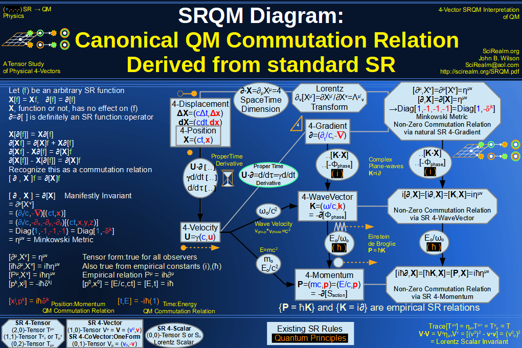
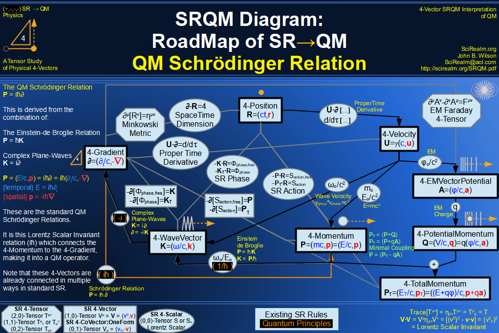
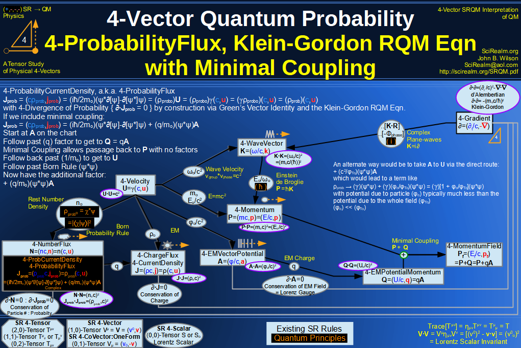
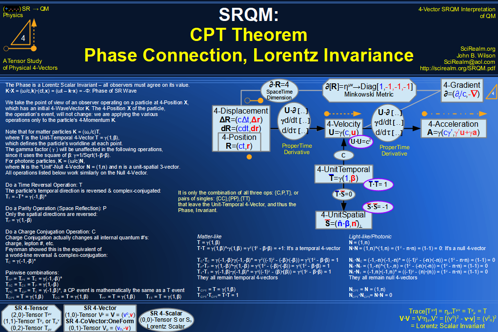
quantum
relativity

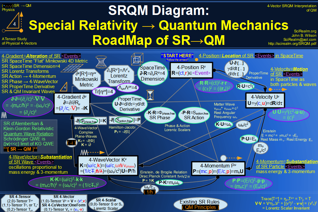
See SRQM: QM from SR - The 4-Vector RoadMap (.html)
See SRQM: QM from SR - The 4-Vector RoadMap (.pdf)


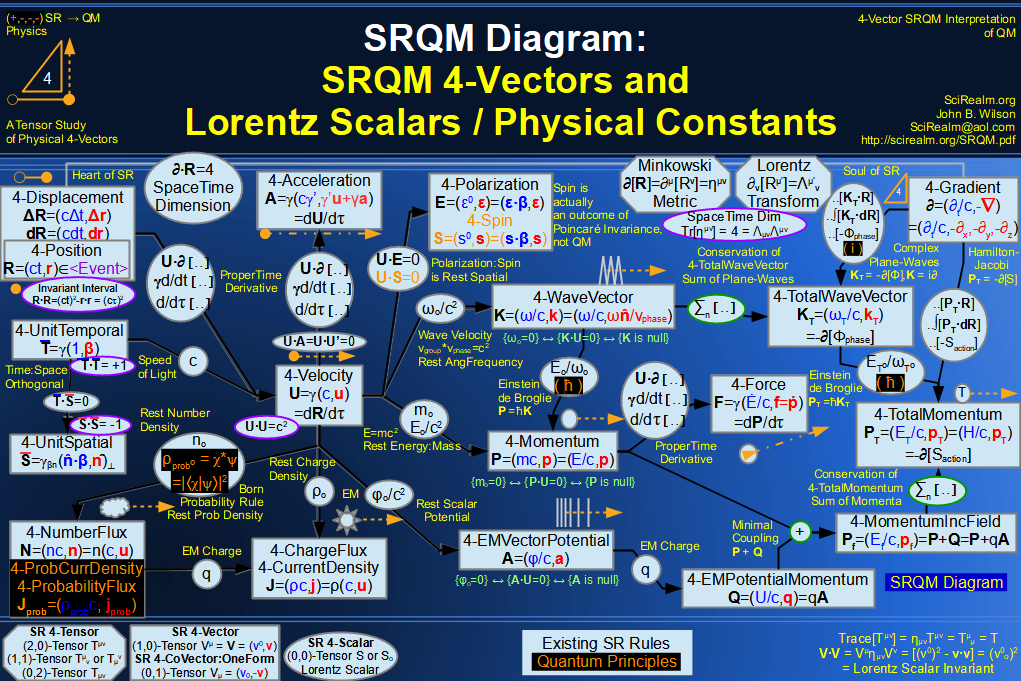
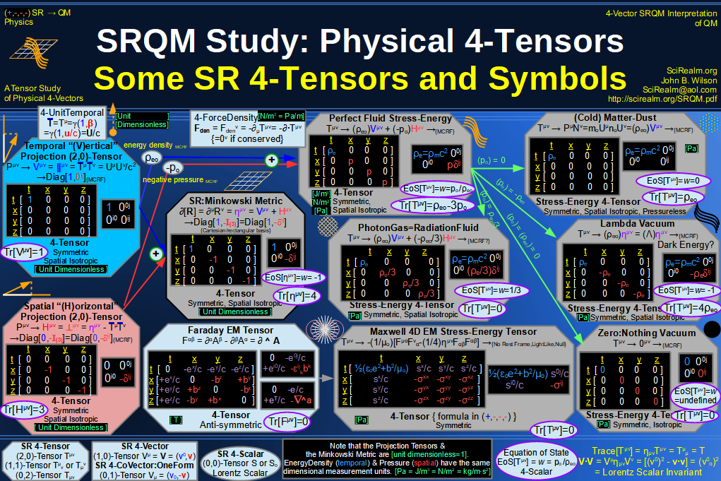
SRQM 4-Vector : Four-Vector and Lorentz Scalar Diagram



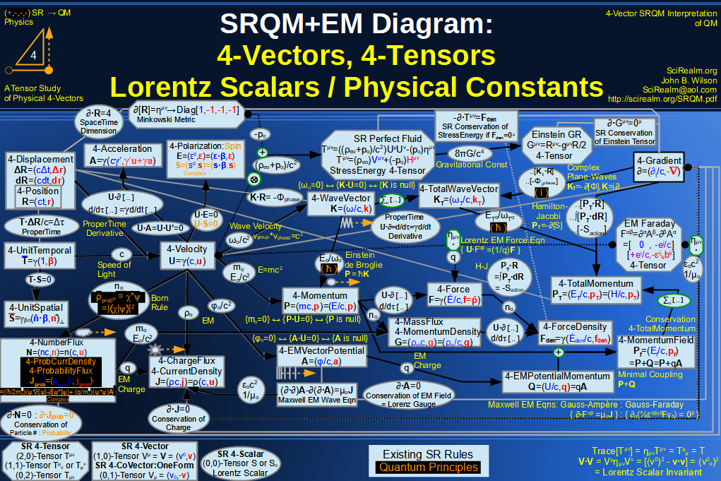
SRQM + EM 4-Vector : Four-Vector and Lorentz Scalar Diagram



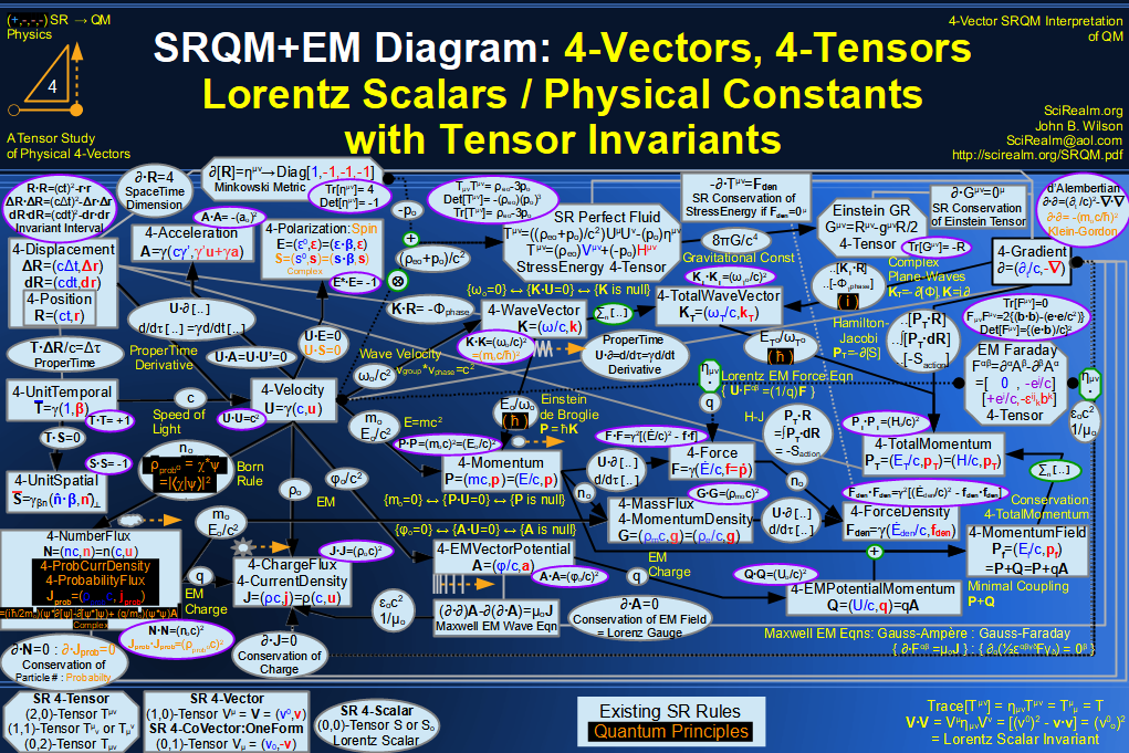
SRQM + EM 4-Vector : Four-Vector and Lorentz Scalar Diagram With Tensor Invariants



SRQM 4-Vector : Four-Vector Stress-Energy & Projection Tensors Diagram



SRQM 4-Vector : Four-Vector SR Quantum RoadMap



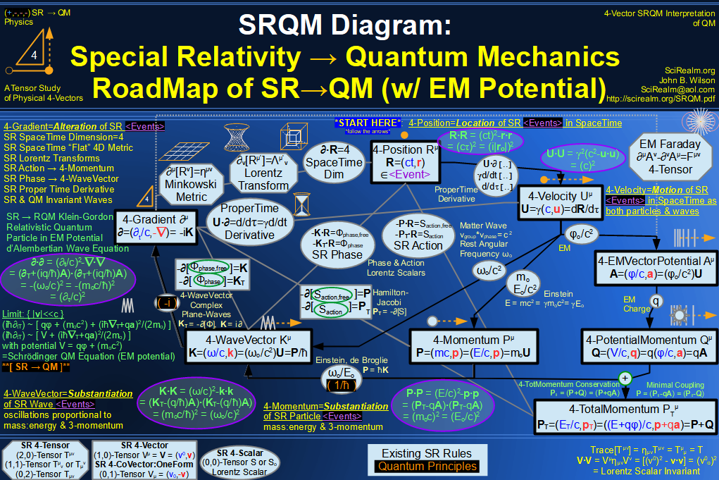
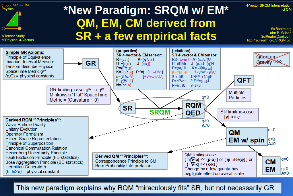
SRQM + EM 4-Vector : Four-Vector SR Quantum RoadMap



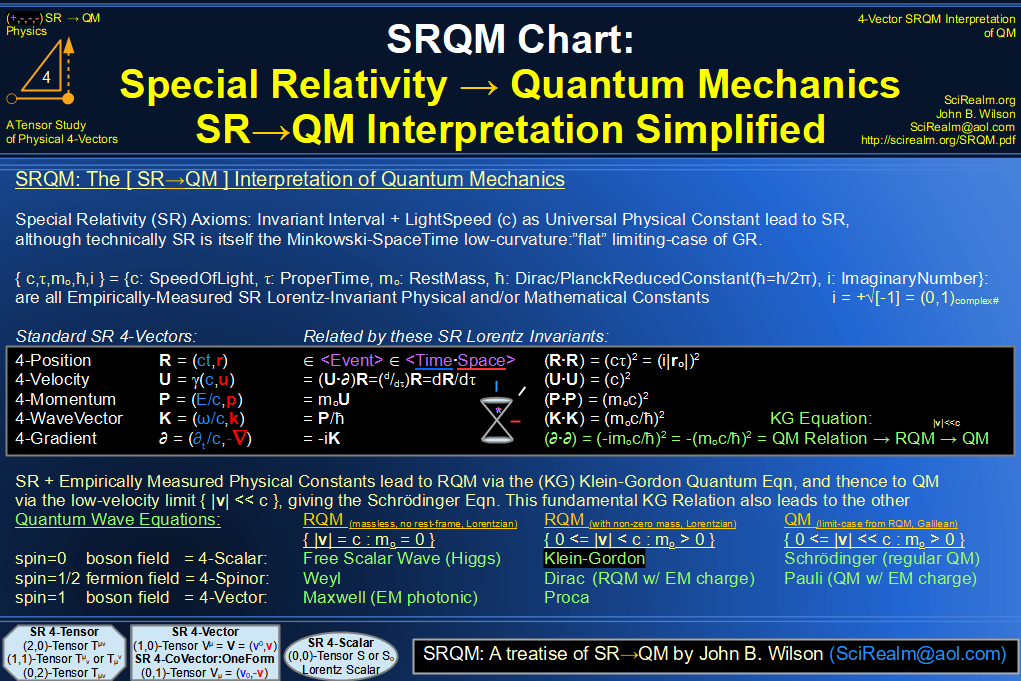
SRQM + EM 4-Vector : Four-Vector SR Quantum RoadMap - Simple



SRQM 4-Vector : Four-Vector New Relativistic Quantum Paradigm



SRQM + EM 4-Vector : Four-Vector New Relativistic Quantum Paradigm (with EM)



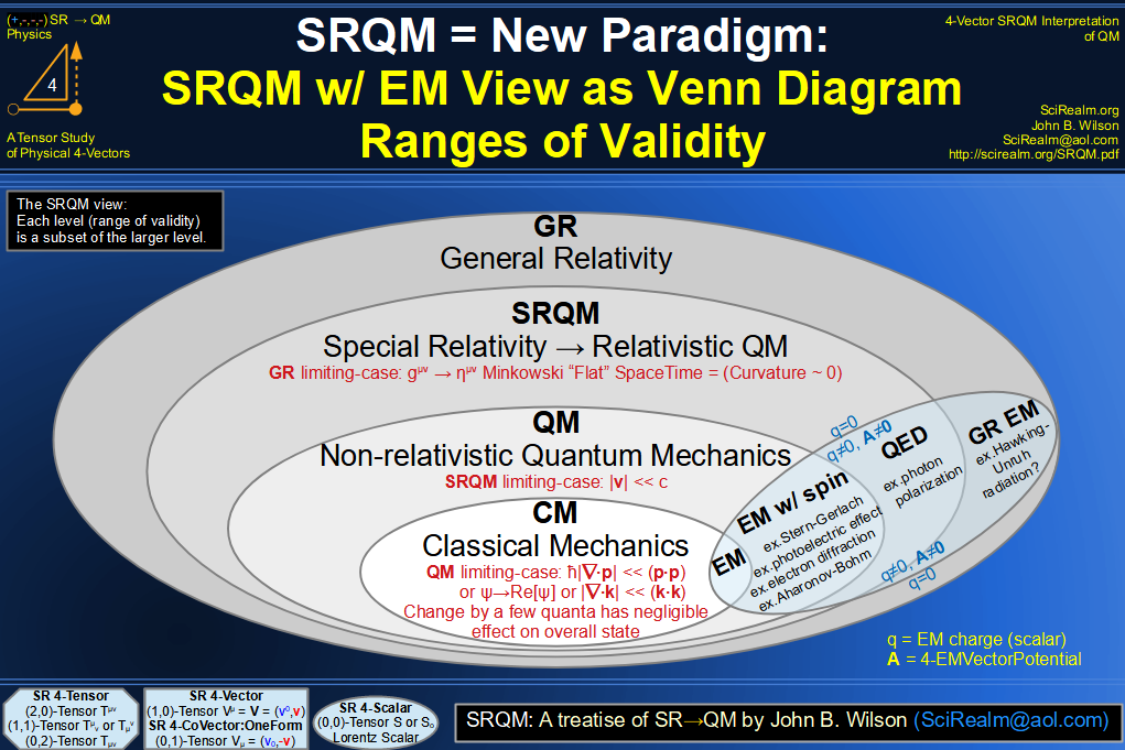
SRQM 4-Vector : Four-Vector New Relativistic Quantum Paradigm - Venn Diagram



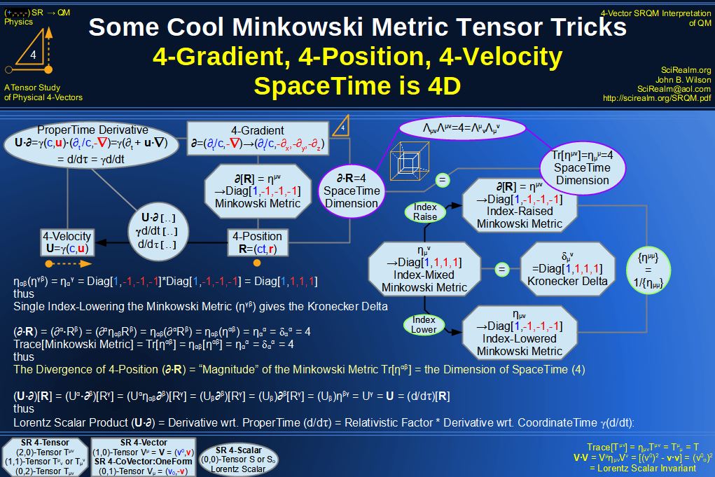
SRQM 4-Vector : Four-Vector SpaceTime is 4D



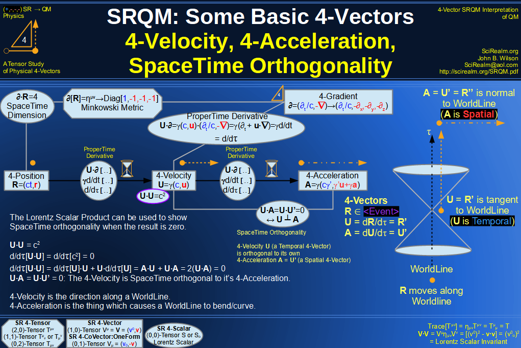
SRQM 4-Vector : Four-Vector SpaceTime Orthogonality



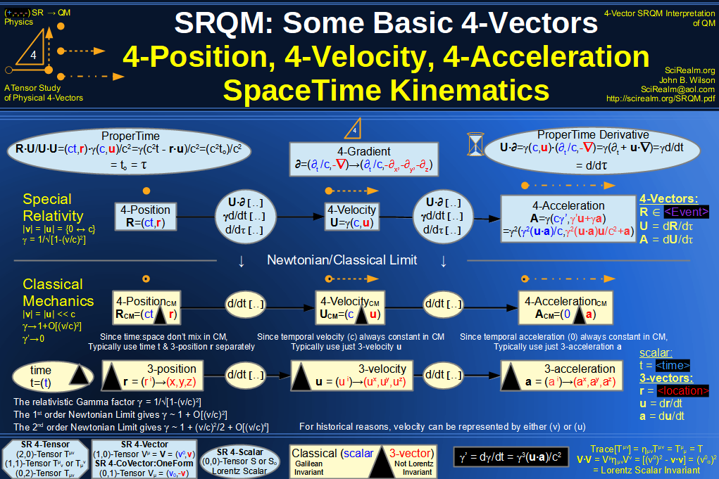
SRQM 4-Vector : Four-Vector 4-Position, 4-Velocity, 4-Acceleration Diagram



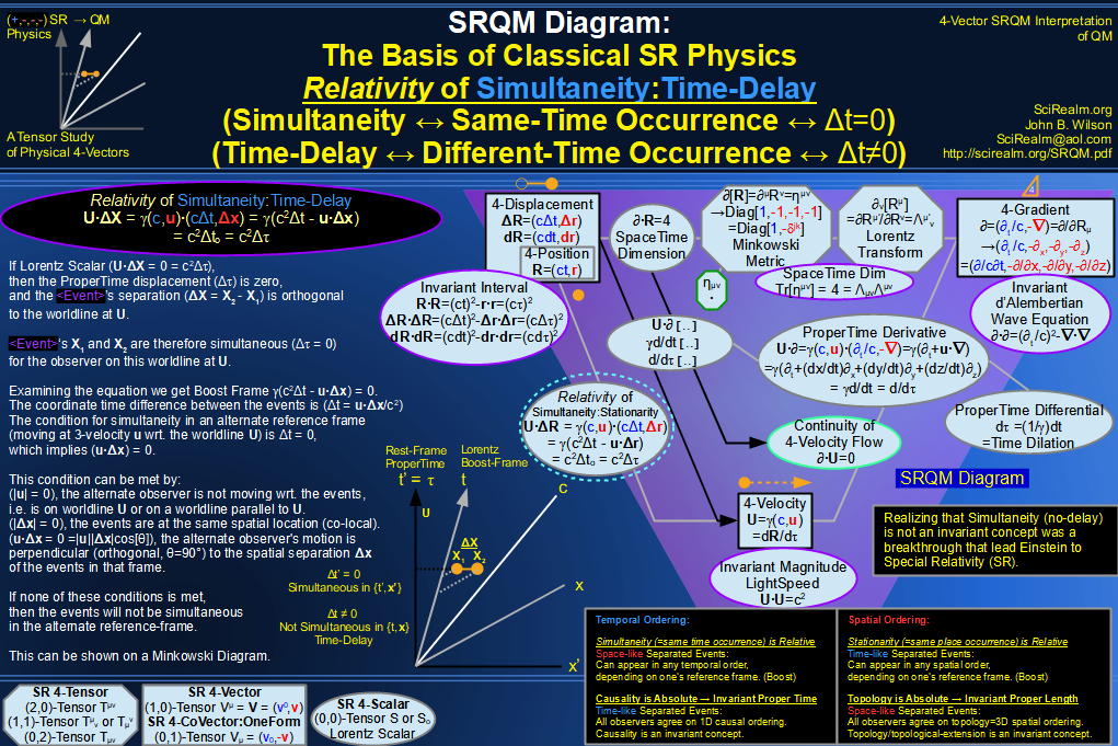
SRQM 4-Vector : Four-Vector 4-Displacement, 4-Velocity, Relativity of Simultaneity Diagram



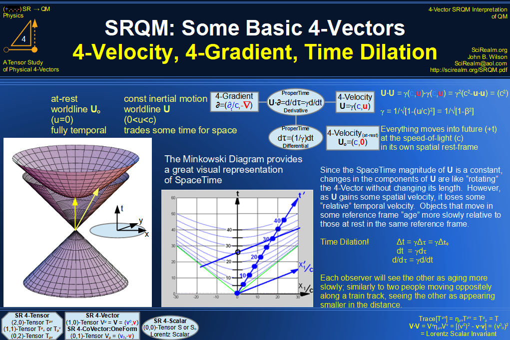
SRQM 4-Vector : Four-Vector 4-Velocity, 4-Gradient, Time Dilation Diagram



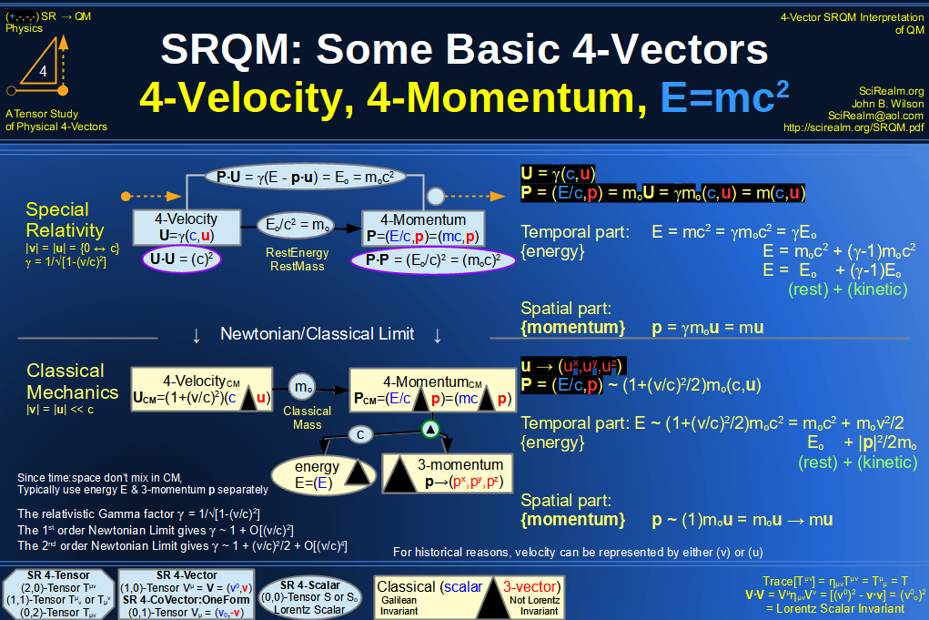
SRQM 4-Vector : Four-Vector 4-Vector, 4-Velocity, 4-Momentum, E=mc^2 Diagram



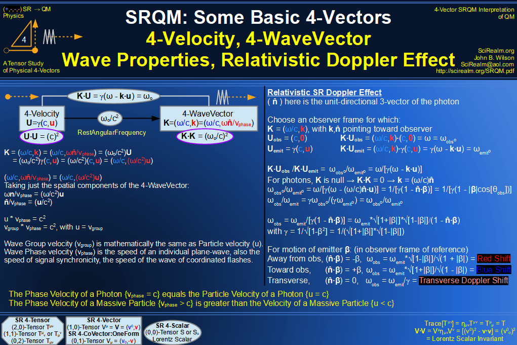
SRQM 4-Vector : Four-Vector 4-Velocity, 4-WaveVector, Relativistic Doppler Effect Diagram



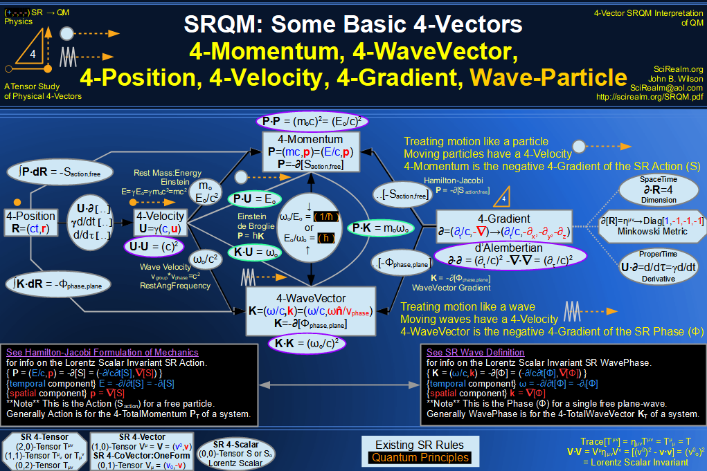
SRQM 4-Vector : Four-Vector Wave-Particle Diagram



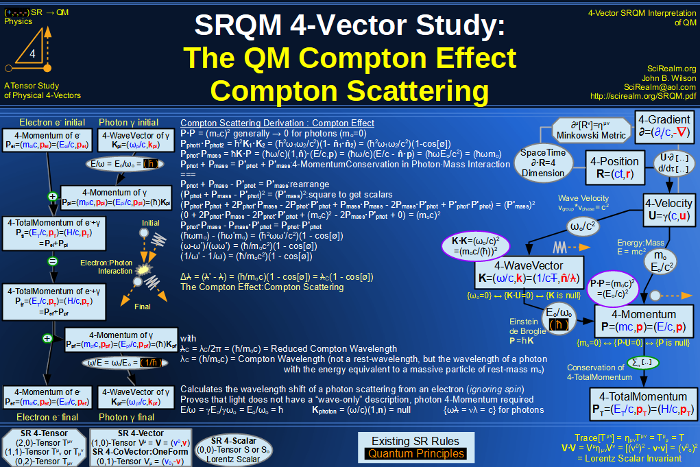
SRQM 4-Vector : Four-Vector Compton Effect Diagram



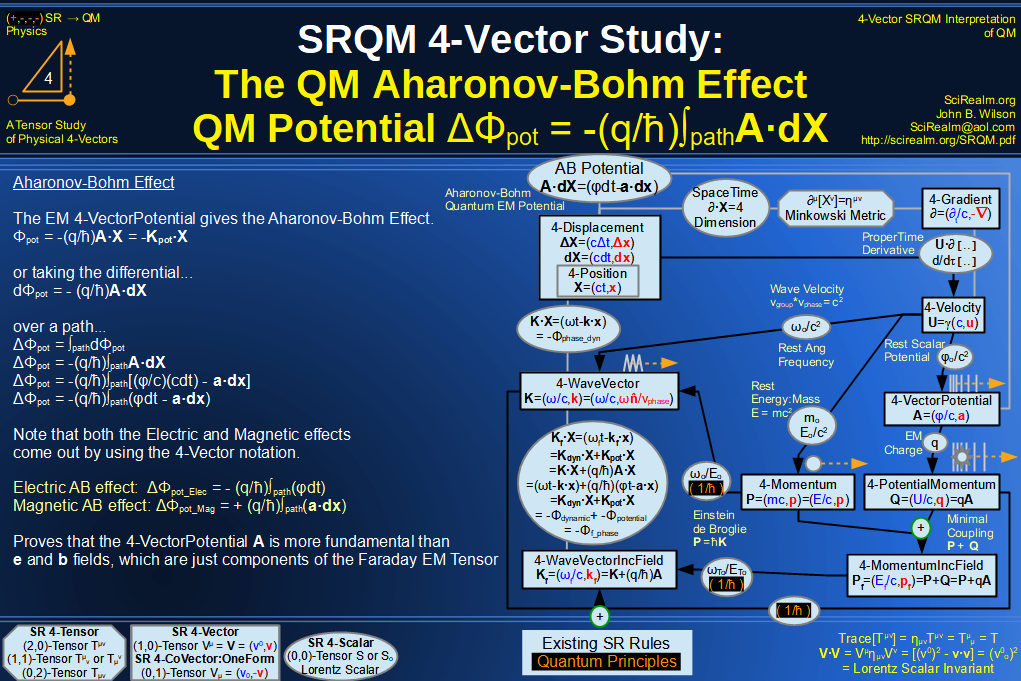
SRQM 4-Vector : Four-Vector Aharonov-Bohm Effect Diagram



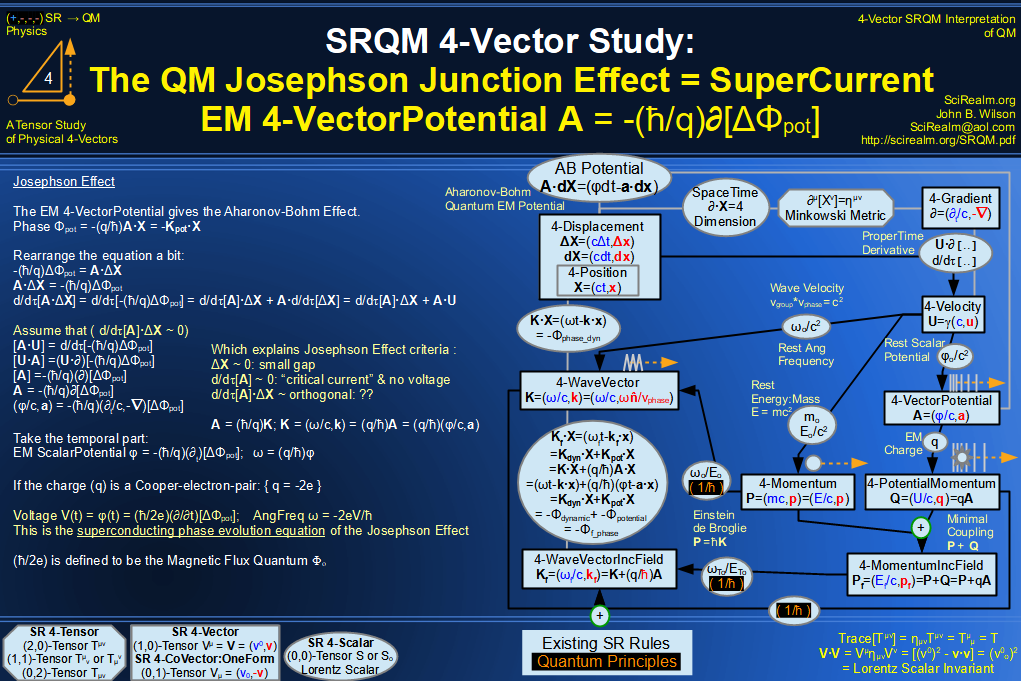
SRQM 4-Vector : Four-Vector Josephson Junction Effect Diagram



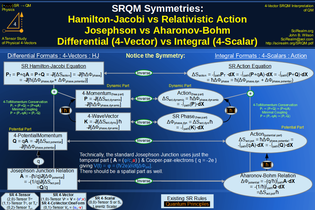
SRQM 4-Vector : Four-Vector Hamilton-Jacobi vs Action, Josephson vs Aharonov-Bohm Diagram



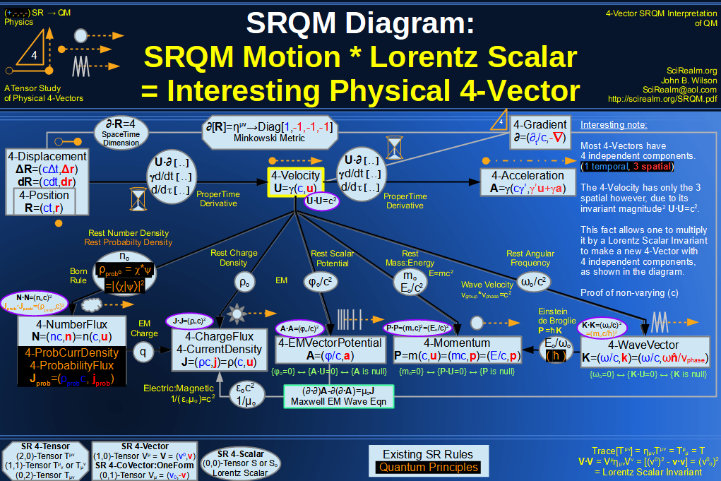
SRQM 4-Vector : Four-Vector Motion of Lorentz Scalar Invariants



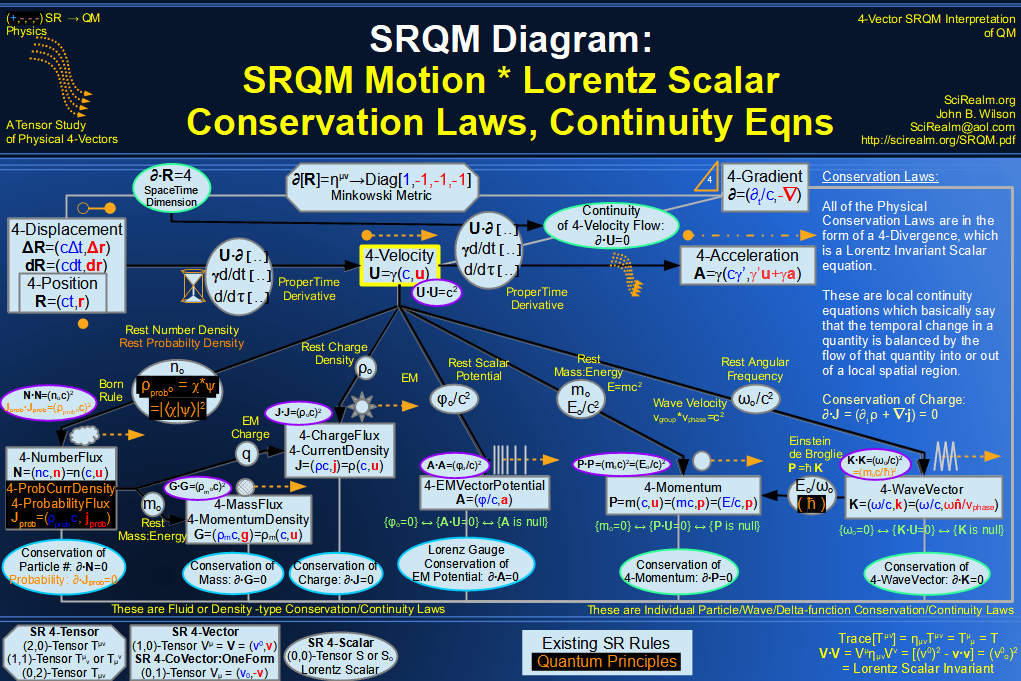
SRQM 4-Vector : Four-Vector Motion of Lorentz Scalar Invariants, Conservation Laws & Continuity Equations



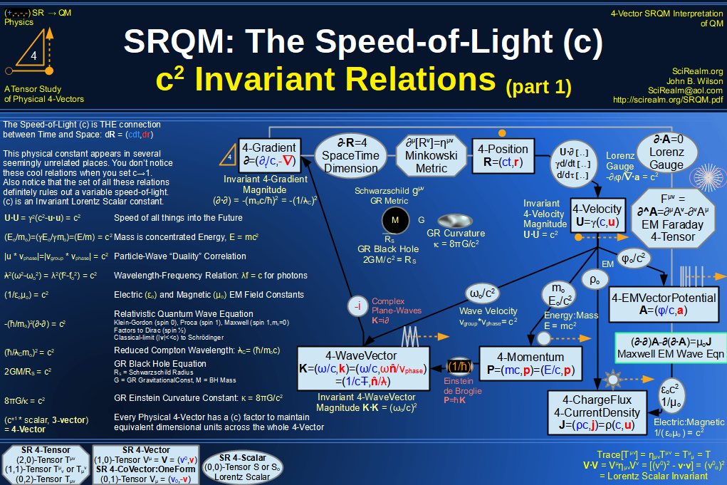
SRQM 4-Vector : Four-Vector Speed of Light (c)



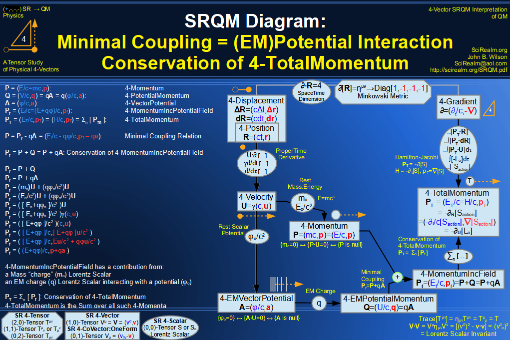
SRQM 4-Vector : Four-Vector Minimal Coupling Conservation of 4-TotalMomentum)



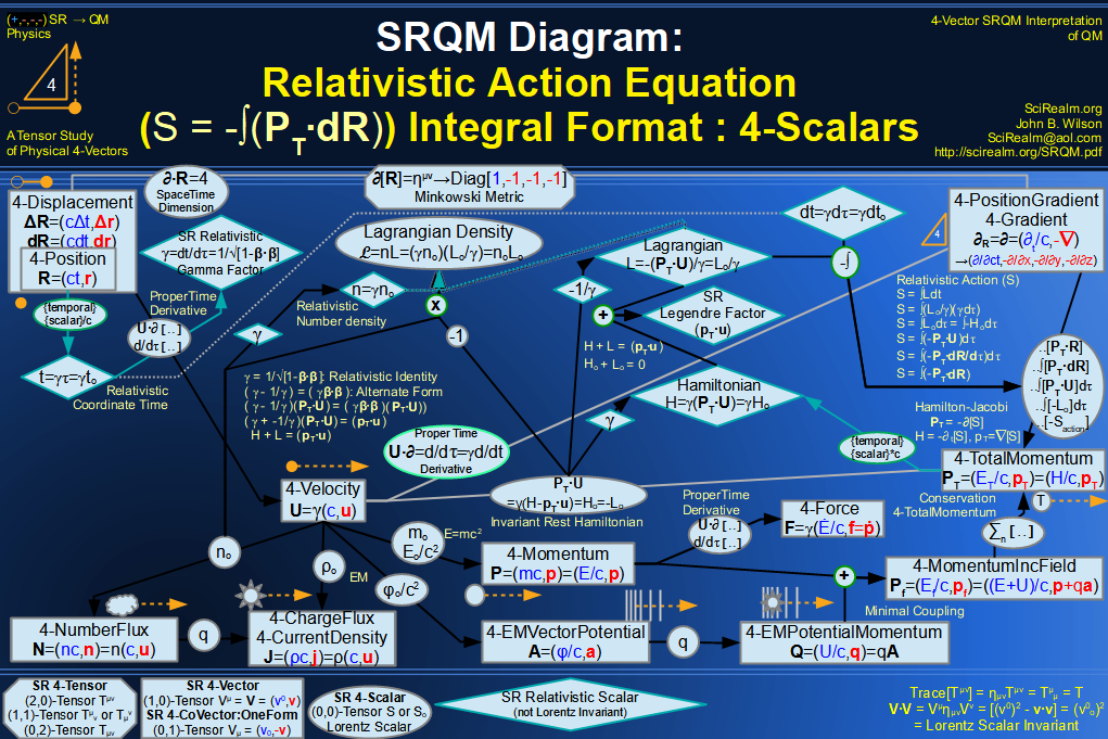
SRQM 4-Vector : Four-Vector Relativistic Action (S) Diagram



SRQM 4-Vector : Four-Vector Relativistic Lagrangian Hamiltonian Diagram



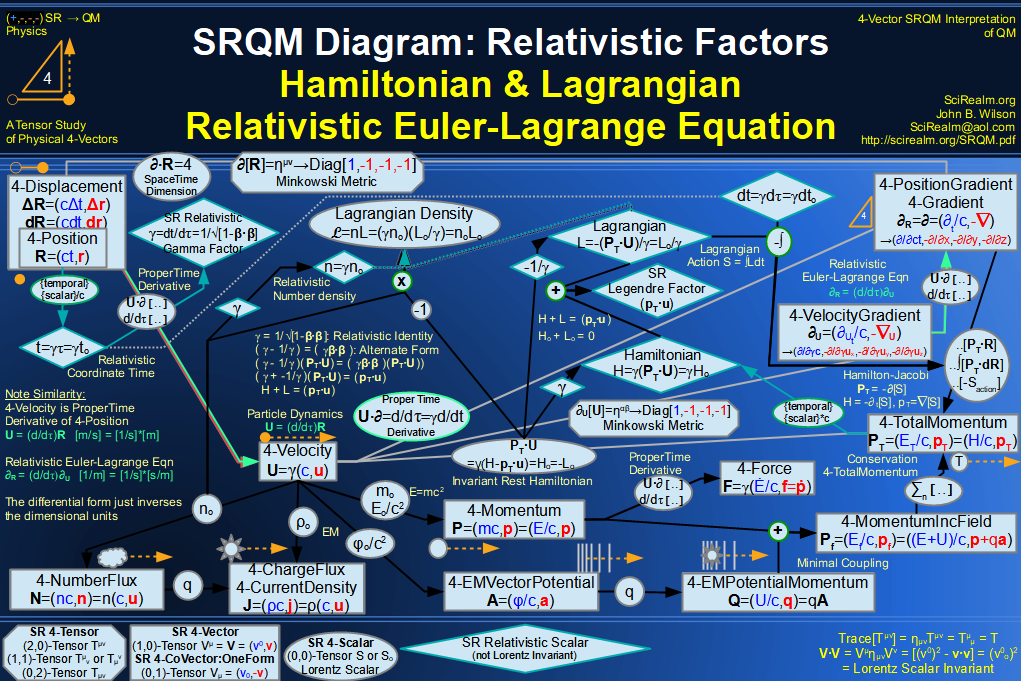
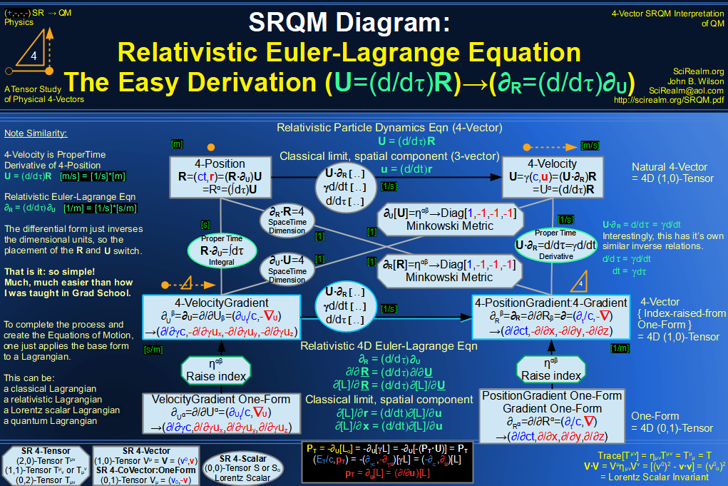
SRQM 4-Vector : Four-Vector Relativistic Euler-Lagrange Equation



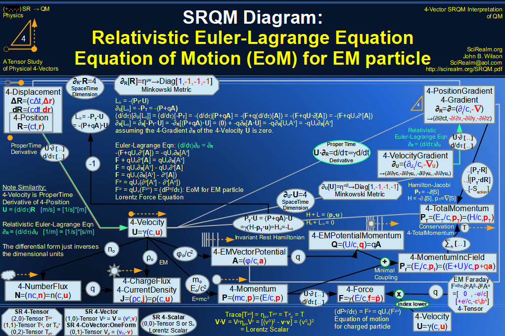
SRQM 4-Vector : Four-Vector Relativistic EM Equations of Motion



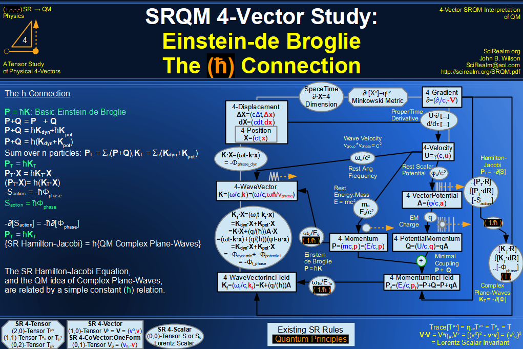
SRQM 4-Vector : Four-Vector Einstein-de Broglie Relation hbar



SRQM 4-Vector : Four-Vector Quantum Canonical Commutation Relation



SRQM 4-Vector : Four-Vector QM Schroedinger Relation



SRQM 4-Vector : Four-Vector Quantum Probability



SRQM 4-Vector : Four-Vector CPT Theorem



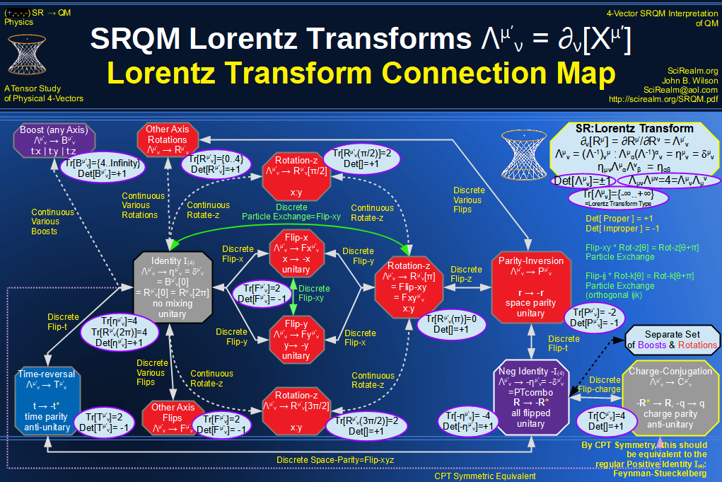
SRQM 4-Vector : Four-Vector Lorentz Transforms Connection Map



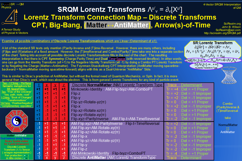
SRQM 4-Vector : Four-Vector Lorentz Discrete Transforms



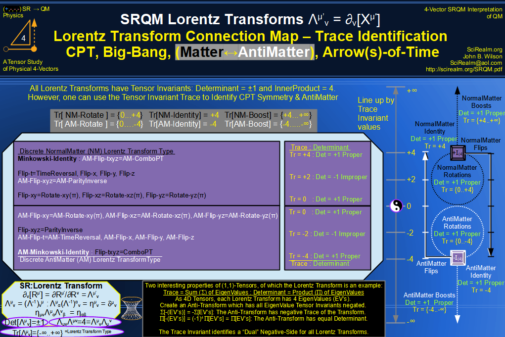
SRQM 4-Vector : Four-Vector Lorentz Transforms - Trace Identification



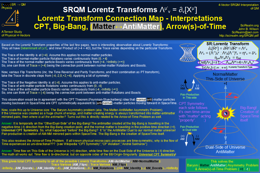
SRQM 4-Vector : Four-Vector Lorentz Lorentz Transforms-Interpretations
CPT Symmetry, Baryon Asymmetry Problem Solution, Matter-Antimatter Symmetry Solution, Arrow-of-Time Problem Solution, Big-Bang!



See SRQM: QM from SR - The 4-Vector RoadMap (.html)
See SRQM: QM from SR - The 4-Vector RoadMap (.pdf)

The Science Realm: John's Virtual Sci-Tech Universe John's Science & Math Stuff: | About John | Send email to John 4-Vectors | Ambigrams | Antipodes | Covert Ops Fragments | Cyrillic Projector | Forced Induction (Sums Of Powers Of Integers) | Fractals | Frontiers | JavaScript Graphics | Kid Science | Kryptos | Philosophy | Photography | Prime Sieve | QM from SR | QM from SR-Simple RoadMap | SR 4-Vector & Tensor Calculator | Quantum Phase | Quotes | RuneQuest Cipher Challenge | Scientific Calculator (complex capable) | Secret Codes & Ciphers | Science+Math | Sci-Pan Pantheist Poems | Stereograms | SuperMagicSqr4x4 | Turkish Grammar |

Quantum Mechanics is derivable from Special Relativity See SRQM - QM from SR - Simple RoadMap (.html) See SRQM - QM from SR - Simple RoadMap (.pdf)